MAS183 Support

• Stats Clinics (starting week two)
• Alethea's office hours
• PASS Classes
• Revision sessions in non-teaching weeks
• Transitioning to MAS183 Worksheets
• Maths support officers available for poor scores on the diagnostic test

Workshop task - Sampling

Using the different sampling methods described in the first lecture, students were asked to sample a sample of 1080 jellybeans (right) to determine the proportion of yellow jellybeans.

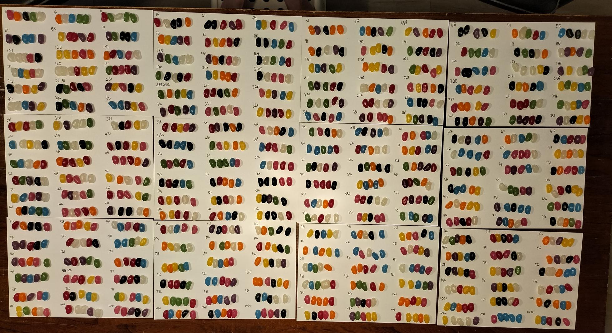
Random sampling method

Calculating the sample proportion was done as follows:

1. Decide on the sample size. 30 to 50 jellybeans was suggested.
2. Use an online simple random sampling applet to get a sample of jelly beans.
3. Count the number of yellow jelly beans in the sample
4. Calculate the proportion using the following equation

Random sampling results

Results were recorded into a csv and the number of yellow jellybeans in a sample of thirty was two, giving it the following proportion $$\hat{p}=\frac{2}{30} =\overline{0.066}$$
or $\mathrm{\%}6.6$

Systemic Sampling method

Calculating the sample proportion was done as follows:

1. Decide on the sample size. 30 to 50 jellybeans was suggested.
2. Use an online simple random sampling applet to get a starting point and record each $yth$ sample.
3. Count the number of yellow jelly beans in the sample
4. Calculate the proportion using the following equation

Systemic sampling results
Result was recorded differently to the method as the random number generator was set to values between one and thirty six, and used to determine both the starting point and $y$ (interval between values). Each sixth sample was recorded, leading to the following proportion:

or $\mathrm{\%}10$

Plotting samples

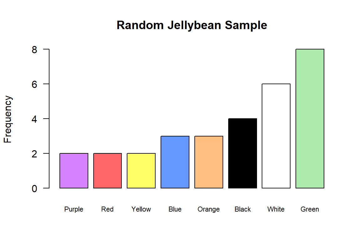
The samples collected were entered into csv files and plotted into bar plots by their corresponding colours.

This is the csv for the simple random sampling

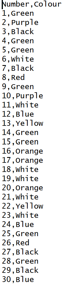
To plot the values, they were sorted into a table using the following command ```

TableName <- table (Dataset$Column)

The resulting frequency table for simple random sampling looked like this

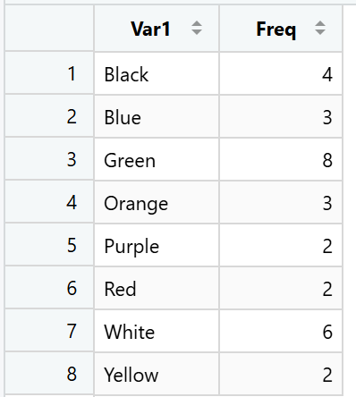
The colours of the bar plot were selected with the following command:

ColourVariableName <- c("#hexcode", "#hexcode", "#hexcode",)
# in formating of table, col=ColourVariableName

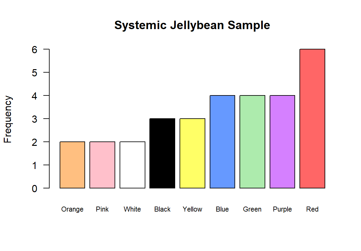
The following are the resulting plots for the frequencies of each sample.
Random sampling

Systemic sampling

next workshop